Runge-Kutta methods of differential equation solvers
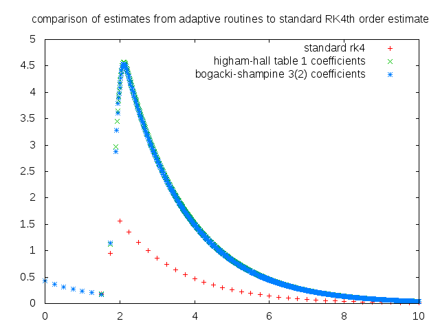
I knew that the difference would be large but not this large. Above is a plot of the estimates from a standard 4th order runge-kutta method compared with two other adaptive runge kutta routines. Adaptive runge-kutta routines vary the step size depending on the difference between mth order and nth order runge-kutta estimates, where m and n are usually 4 and 5. The Cash-Karp implementation of the runge-kutta fehlberg method, which is adaptive in nature, is one of the popular stepper routines in use. Each of these routines compares the error in the estimates from the nth and mth order routines with a preset tolerance and increase or decrease the step size appropriately. The above is a plot of the numerical solution of a first order ODE, the analytical solution to which is a narrow gaussian. And you can clearly see how wrong we are. The gaussian has a center at 2 and a width of 0.075 so one will have to start with a very small value to h to begin with, if one is interested in coming up with a simulation closer to reality. There were a couple of other comments made on my code so I guess we have a full plate.