Week 3 - PYTHON!!! and Data Analysis.
Yes. The exclamation marks, all of three of them are necessary!
Because i cannot tell you in words how blown away i am having used python for the last week. Don't get me wrong, i've used/tried python before, learning for a couple of days but eventually abandoning it! And the reason i love (yes, love. not just like. ever-lasting love) it so much is because of what i've been able to accomplish. Before i start with what happened this week, I'm sure there are ways to do the same using other programming languages : C, Java, Mathematica and what not but they (probably) don't have the extremely extensive documentation and gazillions of examples.
So, as I said last week, my work for the summer was the reproduce the results of a certain paper by Richards, Gordon T (2000) which analyses the color-redshift relation of 2625 quasars. I've extensively explained the details of the paper and the results i am to reproduce in last week's post. And as i said, last week ended with data in hands, acquired from the SDSS archive through SQL Query, which i was to refine and analyze. There are actually 2 data sets i worked on, one is a data set of ~900 quasars, part of the original 2625 quasars analyzed in the paper and the second one what what i acquired from the SDSS.
The original data set came with a README file, which gave me this information -
Byte-by-byte Description of file: table2.dat
--------------------------------------------------------------------------------
Bytes Format Units Label Explanations
--------------------------------------------------------------------------------
1- 30 A30 --- Name Quasar name
32- 36 F5.3 --- z Redshift
38- 39 I2 h RAh Right Ascension (J2000)
51- 52 I2 deg DEd Declination (J2000)
67- 71 F5.2 mag u*mag The SDSS u* band photometry (1)
79- 83 F5.2 mag g*mag The SDSS g* band photometry (1)
91- 95 F5.2 mag r*mag The SDSS r* band photometry (1)
103-107 F5.2 mag i*mag The SDSS i* band photometry (1)
115-119 F5.2 mag z*mag The SDSS z* band photometry (1)
i removed a couple of the lines from the file but well that was the part of the file that i needed! And let me tell you now why this readme file was necessary! When i started using python to extract the information from this .dat file, each lines was stored as a string, a string where the bits 32:36 are the red shift of the object and so on. You get the point. So, in order to extract the red shift from each of these strings, i needed to know the exact byte location of the different columns i needed to extract. Again, i'm sure i'd have eventually figured out what the structure of the file is but hey, this made my life easier.
Moral of the story : Have README files. in each and every directory. For your sake and for someone else's sake who might be using your system or your data later on.
so, once i'd extracted the red shift and the 5 magnitudes, i calculated the 4 colors - u-g, g-r, r-i, i-z - if you don't understand what i mean by color, go read last week's post! and then i go about plotting the a histogram of the redshift and the colors as a fn of redshift.
Here's how they looks like -


I'd say they came out pretty good, you can compare them from the original plots, you can check them from the previous post! So, as you can see, the color-red shift relation isn't random, there is a clear relation between the color of a quasar and the red shift it is at! All 4 of the colors show a beautiful evolution.
Now, we go about calculating the median redshift of each of these colors.
We take bins at intervals of 0.05 on the x axis - the red shift - where the bin width is 0.075. Now, we look at all of the quasars in this bin and calculate the median color for these quasars. Once we've done the same for all of the bins, we plot the median color against red shift.
Here's how that looks like -
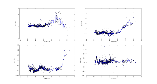
The blue line you see is the median color - redshift relation.
Now, let's get to why i'm doing all of this!
As i've said the last time, ted shifts of quasars are obtained by studying the spectra of these objects. And spectroscopy is in general very time taking, in comparison to photometry of the quasar. So, if there is a method to estimate the red shift of a quasar using just photometry, then it'd make life simpler. Also, by estimating a quasar's red shifts using photometry (called PhotoZ from hereon), we can better select candidates that need to be studied using spectroscopy - quasars with high estimated PhotoZ can be selected for spectroscopy instead of having to study each quasar! It basically makes our object selection more efficient!
Estimating PhotoZ, as you probably see by now, i done by looking at where a quasar falls in the 4 color-red shift plots above.
So, that's the year 2000. This telescope has been observing day and night (ohh wait, telescopes can't observe in the day, unless they're radio telescopes) and identifying more and more quasars. The quasar count this time is ~300,000 and the # of quasars whose red shift has been calculated using spectroscopy is ~150,000! Now, i'm basically trying to replicate the same process i mentioned above - calculating color, plotting color-red shift and calculating median color - with data on the ~150,000 quasars!
And the reason why i was talking about the README file in the previous case is because the new data is in a .csv format, it did NOT come with a readme file and it was a bitch to look for ways to open and extract useful information out of it!
Anyway, here's how the preliminary results look like -
(i'm running the code to calculate the median colors as i write)


Because i cannot tell you in words how blown away i am having used python for the last week. Don't get me wrong, i've used/tried python before, learning for a couple of days but eventually abandoning it! And the reason i love (yes, love. not just like. ever-lasting love) it so much is because of what i've been able to accomplish. Before i start with what happened this week, I'm sure there are ways to do the same using other programming languages : C, Java, Mathematica and what not but they (probably) don't have the extremely extensive documentation and gazillions of examples.
So, as I said last week, my work for the summer was the reproduce the results of a certain paper by Richards, Gordon T (2000) which analyses the color-redshift relation of 2625 quasars. I've extensively explained the details of the paper and the results i am to reproduce in last week's post. And as i said, last week ended with data in hands, acquired from the SDSS archive through SQL Query, which i was to refine and analyze. There are actually 2 data sets i worked on, one is a data set of ~900 quasars, part of the original 2625 quasars analyzed in the paper and the second one what what i acquired from the SDSS.
The original data set came with a README file, which gave me this information -
Byte-by-byte Description of file: table2.dat
--------------------------------------------------------------------------------
Bytes Format Units Label Explanations
--------------------------------------------------------------------------------
1- 30 A30 --- Name Quasar name
32- 36 F5.3 --- z Redshift
38- 39 I2 h RAh Right Ascension (J2000)
51- 52 I2 deg DEd Declination (J2000)
67- 71 F5.2 mag u*mag The SDSS u* band photometry (1)
79- 83 F5.2 mag g*mag The SDSS g* band photometry (1)
91- 95 F5.2 mag r*mag The SDSS r* band photometry (1)
103-107 F5.2 mag i*mag The SDSS i* band photometry (1)
115-119 F5.2 mag z*mag The SDSS z* band photometry (1)
i removed a couple of the lines from the file but well that was the part of the file that i needed! And let me tell you now why this readme file was necessary! When i started using python to extract the information from this .dat file, each lines was stored as a string, a string where the bits 32:36 are the red shift of the object and so on. You get the point. So, in order to extract the red shift from each of these strings, i needed to know the exact byte location of the different columns i needed to extract. Again, i'm sure i'd have eventually figured out what the structure of the file is but hey, this made my life easier.
Moral of the story : Have README files. in each and every directory. For your sake and for someone else's sake who might be using your system or your data later on.
so, once i'd extracted the red shift and the 5 magnitudes, i calculated the 4 colors - u-g, g-r, r-i, i-z - if you don't understand what i mean by color, go read last week's post! and then i go about plotting the a histogram of the redshift and the colors as a fn of redshift.
Here's how they looks like -
NOTE : you could open the images in a new tab, to see the details better.


I'd say they came out pretty good, you can compare them from the original plots, you can check them from the previous post! So, as you can see, the color-red shift relation isn't random, there is a clear relation between the color of a quasar and the red shift it is at! All 4 of the colors show a beautiful evolution.
Now, we go about calculating the median redshift of each of these colors.
We take bins at intervals of 0.05 on the x axis - the red shift - where the bin width is 0.075. Now, we look at all of the quasars in this bin and calculate the median color for these quasars. Once we've done the same for all of the bins, we plot the median color against red shift.
Here's how that looks like -

The blue line you see is the median color - redshift relation.
Now, let's get to why i'm doing all of this!
As i've said the last time, ted shifts of quasars are obtained by studying the spectra of these objects. And spectroscopy is in general very time taking, in comparison to photometry of the quasar. So, if there is a method to estimate the red shift of a quasar using just photometry, then it'd make life simpler. Also, by estimating a quasar's red shifts using photometry (called PhotoZ from hereon), we can better select candidates that need to be studied using spectroscopy - quasars with high estimated PhotoZ can be selected for spectroscopy instead of having to study each quasar! It basically makes our object selection more efficient!
Estimating PhotoZ, as you probably see by now, i done by looking at where a quasar falls in the 4 color-red shift plots above.
So, that's the year 2000. This telescope has been observing day and night (ohh wait, telescopes can't observe in the day, unless they're radio telescopes) and identifying more and more quasars. The quasar count this time is ~300,000 and the # of quasars whose red shift has been calculated using spectroscopy is ~150,000! Now, i'm basically trying to replicate the same process i mentioned above - calculating color, plotting color-red shift and calculating median color - with data on the ~150,000 quasars!
And the reason why i was talking about the README file in the previous case is because the new data is in a .csv format, it did NOT come with a readme file and it was a bitch to look for ways to open and extract useful information out of it!
Anyway, here's how the preliminary results look like -
(i'm running the code to calculate the median colors as i write)

the 4 color-redshift plots

enhanced -

the median u-g color vs red shift. Partial plot. Further work needed here.

I'll write about the different python libraries i've come across over the week, in search of ways to read and analyse the files (the original .dat and the new .csv) in a separate post but well, that's all for now.
In the mean while, try figure out how to calculate the median color. To elaborate, let's say i have a file with 2 columns * 898 rows worth of data - one is the color and the second is the redshift. To note, the columns aren't ordered - neither by color nor by red shift. The range of red shifts though is 0-5.
Now, as i mentioned, take bins at red shift intervals of 0.05 whose size is 0.075
(yes, two consecutive bins do overlap! don't ask me why i chose this size, it's from the paper!)
and extract all of the quasars in this red shift bin. calculate their median color and move on to the next bin. There is a brute force way to do this, which i'm running right now cos i need results right now. And then there's an elegant way i'm trying to code. Let's see if it works cos OHMYGOD the brute force is taking too long!
So, there you go.
Work so far this week.
Later...