Colors of Quasars- Data Acquisition and Analysis
Over the course of my project, i've had to work with multiple data sets. Two of the important data sets were the original data set used by Richards et al in their paper and a new data set that i acquired - data set whose samples are constrained by the same conditions as mentioned in the richards et al paper.
Part of the original data used in the paper can be acquired from browsed from the vizier archived data, SIMBAD object list and NED object list. These data sets can be found through a simple search for the paper on SAO/NASA ADS.
As mentioned, this is just a part of the original data set i.e data pertaining to only 898 of the 2625 quasars used in the original paper are available for download through these links. The location for the rest of the sample set is still elusive - maybe they were released as part of the SDSS Data Release 1 which is why they weren't specifically included in this data set. This conclusion is based on the fact that none of these 898 objects are classified as SDSS - although SDSSp doesn't appear here and there.
The new data set was acquired by querying the Data Release 9 using an SQL Query. Constraints defined in the original paper were applied while querying DR9. A total of 146,659 query were found to satisfy the query.
The AB magnitude constraints set in the original paper are
The SQL query used to retrieve the new data set -
A sample of how the data looks -
This new data has been uploaded to my google drive and is available for download. Note that the file is 16.4 MB in size. You can query the DR9 of SDSS yourself
here.
Analysis of the data sets was done using Python. There are two data sets - the original data set which has a .dat file extension and the new data set which has a .csv file extension.
The .dat file has been extracted as follows -
Byte-by-byte Description of file: table2.dat
Note
Data extracted has been visualized as -


Similarly, the new data set has been read using the pandas library


Though it is not obvious, you can see that the color-redshift plots for quasars from the old sample set and for those from the new sample set follow a similar pattern wrt red shift!
We are now interested in obtaining a median color vs redshift relation for each of the 4 colors - u-g, g-r, r-i, i-z.
The motivation behind using the median color instead of a mean color is due to the presence of a large number of outliers in our data set - outliers in the form of reddened quasars, seyfert galaxies & broad emission line (BAL) quasars, outliers which may skew the mean.
Following the paper 'Photometric Redshifts of Quasars' by Richards et al 2001, for each of the 4 colors - the red shift range is first binned with centers at0.05 redshift intervals with a bin width of 0.075 for z ≤2.15 , 0.2 for 2.15≤z≤2.5 and 0.5 for z>2.5 centered at the 0.05. We now calculate the median colors for all of the quasars lying within these bins.
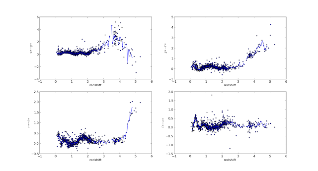
Here, the median color has been calculated using a bin width of 0.05 over the whole red shift interval. As you can see, the median color plotted in turquoise varies sharply beyondz=3 . The reason for this, i believe, is because of the rapid fall in the number of quasars available in the red shift bins beyond this redshift, as is obvious from the histogram shown above! And I speculate that this is the reason why the authors chose aforementioned bin values.
Thus, I've been able to partially replicate and extend the paper richards et al 2001.
Further, having extended the results to a new sample set with 146,659 quasars, interesting features can be seen in the color-redshift plots. Vertical clustering of quasar colors can be seen in the color redshift plots of the new data set - clustering indicative of a wide color range for quasars at roughly the same redshift. Three such features are clearly visible in the u-g color vs redshift plot - at z~1, z~1.3 and z~1.6. Some of these features are visible in the other color-redshift plots.
Looking at the spatial projection, it can be seen that most of these quasars fall into two specific clusters. These fields are being further investigated as to understand their peculiar properties.


the function read() should be in
Written with StackEdit.
Part of the original data used in the paper can be acquired from browsed from the vizier archived data, SIMBAD object list and NED object list. These data sets can be found through a simple search for the paper on SAO/NASA ADS.
As mentioned, this is just a part of the original data set i.e data pertaining to only 898 of the 2625 quasars used in the original paper are available for download through these links. The location for the rest of the sample set is still elusive - maybe they were released as part of the SDSS Data Release 1 which is why they weren't specifically included in this data set. This conclusion is based on the fact that none of these 898 objects are classified as SDSS - although SDSSp doesn't appear here and there.
The new data set was acquired by querying the Data Release 9 using an SQL Query. Constraints defined in the original paper were applied while querying DR9. A total of 146,659 query were found to satisfy the query.
The AB magnitude constraints set in the original paper are
The reason behind setting these constraints might be to increase the efficiency of the photo-z estimation. As mentioned, the photo-z method isn't a particularly new method and it's effectiveness depends highly on accurate photometry of the objects. Therefore, the less accurate the photometry, the less accurate the photo-z estimation. Depending on the telescope's physical limitations, the authors might've concluded that the error in photometry for objects beyond these AB magnitude limits is too large.
- u - 22.3
- g - 22.6
- r - 22.7
- i - 22.4
- z - 20.5
The SQL query used to retrieve the new data set -
select
    plateX.plate, plateX.mjd, specObj.fiberID,

    PhotoObj.modelMag_u, PhotoObj.modelMag_g,
    PhotoObj.modelMag_r, PhotoObj.modelMag_i, PhotoObj.modelMag_z,
    PhotoObj.ra, PhotoObj.dec,

    specObj.z, PhotoObj.ObjID

from
    PhotoObj, specObj, plateX

where
    specObj.bestObjid = PhotoObj.ObjID
    AND plateX.plateID = specObj.plateID
    AND specObj.class = 'qso'
    AND specObj.zWarning = 0
    AND PhotoObj.modelMag_u < 22.3
    AND PhotoObj.modelMag_g < 22.6
    AND PhotoObj.modelMag_r < 22.7
    AND PhotoObj.modelMag_i < 22.4
AND PhotoObj.modelMag_z < 20.5A sample of how the data looks -
| plate | mjd | fiberID | ra | dec | z | ObjID | |||||
|---|---|---|---|---|---|---|---|---|---|---|---|
| 1257 | 52944 | 91 | 19.02 | 16.99 | 15.85 | 15.26 | 14.87 | 71.32 | 25.64 | 0.967008 | 1237660760537100000 |
| 4997 | 55738 | 704 | 21.68 | 20.67 | 19.95 | 19.76 | 19.51 | 256.87 | 32.02 | 0.969408 | 1237655501888550000 |
| 1251 | 52964 | 27 | 20.06 | 17.89 | 16.65 | 15.99 | 15.57 | 66.13 | 27.99 | 0.967218 | 1237660553302510000 |
| 1256 | 52902 | 470 | 19.85 | 17.72 | 16.50 | 15.85 | 15.44 | 69.05 | 25.90 | 0.967194 | 1237660559209400000 |
| 1251 | 52964 | 24 | 19.74 | 17.70 | 16.57 | 16.00 | 15.67 | 65.83 | 28.24 | 0.96773 | 1237660750872310000 |
Analysis of the data sets was done using Python. There are two data sets - the original data set which has a .dat file extension and the new data set which has a .csv file extension.
The .dat file has been extracted as follows -
>>> fin = open('foo.dat')
>>> data = fin.readlines()
>>> fin.close()Byte-by-byte Description of file: table2.dat
| Bytes | Format | Units | Label | Explanations |
|---|---|---|---|---|
| 1- 30 | A30 | Name | Quasar name | |
| 32- 36 | F5.3 | z | Redshift | |
| 38- 39 | I2 | h | RAh | Right Ascension (J2000) |
| 41- 42 | I2 | min | RAm | Right Ascension (J2000) |
| 44- 48 | F5.2 | s | RAs | Right Ascension (J2000) |
| 50 | A1 | DE- | Sign of the Declination (J2000) | |
| 51- 52 | I2 | deg | DEd | Declination (J2000) |
| 54- 55 | I2 | arcmin | DEm | Declination (J2000) |
| 57- 60 | F4.1 | arcsec | DEs | Declination (J2000) |
| 62- 65 | F4.2 | arcsec | DelPos | Difference between SDSS and cataloged positions |
| 67- 71 | F5.2 | mag | The SDSS |
|
| 73- 77 | F5.3 | mag | Uncertainty in umag | |
| 79- 83 | F5.2 | mag | The SDSS |
|
| 85- 89 | F5.3 | mag | Uncertainty in gmag | |
| 91- 95 | F5.2 | mag | The SDSS |
|
| 97-101 | F5.3 | mag | Uncertainty in rmag | |
| 103-107 | F5.2 | mag | The SDSS |
|
| 109-113 | F5.3 | mag | Uncertainty in imag | |
| 115-119 | F5.2 | mag | The SDSS |
|
| 121-125 | F5.3 | mag | Uncertainty in zmag | |
| 127-130 | F4.2 | mag | RedVec | Reddening vector in |
| 132-134 | A3 | Source catalog of each object (3) |
using this, we can extract the relevant columns as
- SDSS magnitudes are based on the AB magnitude system Oke & Gunn (1983ApJ...266..713O), and are given as asinh magnitudes Lupton, Gunn, & Szalay (1999AJ....118.1406L).
- As determined from Schlegel et al. (1998ApJ...500..525S).
- Source catalog of each object -1 = NED -2 = SDSS.
>>> data[i][31:36]
# to extract red shift
>>> data[i][66:71]
# to  extract the u band magnitude
>>> u, g, r, i, z = [], [], [], [], []
>>> redshift = []
>>> for j in xrange(len(data)):
... tmp = data[j][31:36]
... redshift.append(tmp)
... tmp = data[j][31:36]
... u.append(tmp)
... tmp = data[j][78:83]
... g.append(tmp)
... tmp = data[j][90:95]
... r.append(tmp)
... tmp = data[j][102:107]
... i.append(tmp)
... tmp = data[j][114:119]
... z.append(tmp)
...
>>> u_g, g_r, r_i, i_z = [], [], [], []
>>> for j in xrange(len(redshift)):
... tmp = u[j] - g[j]
... u_g.append(tmp)
... tmp = g[j] - r[j]
... g_r.append(tmp)
... tmp = r[j] - i[j]
... r_i.append(tmp)
... tmp = i[j] - z[j]
... i_z.append(tmp)
...
>>> subplot(221)
>>> scatter(redshift, u_g, s=5)
>>> subplot(222)
>>> scatter(redshift, g_r, s=5)
>>> subplot(223)
>>> scatter(redshift, r_i, s=5)
>>> subplot(224)
>>> scatter(redshift, i_z, s=5)Data extracted has been visualized as -
Similarly, the new data set has been read using the pandas library
>>> import pandas as pd
>>> data = pd.read_csv('foo.csv')
>>> data['column_name']
# prints the data in the specific column.
>>> data
# a summary of the data set, including the column identifiers.
<class 'pandas.core.frame.DataFrame'>
Int64Index: 146659 entries, 0 to 146658
Data columns (total 12 columns):
plate         146659  non-null values
mjd           146659  non-null values
fiberID       146659  non-null values
modelMag_u    146659  non-null values
modelMag_g    146659  non-null values
modelMag_r    146659  non-null values
modelMag_i    146659  non-null values
modelMag_z    146659  non-null values
ra            146659  non-null values
dec           146659  non-null values
z             146659  non-null values
ObjID         146659  non-null values
dtypes: float64(8), int64(4)
>>> u,g,r,i,z = data['modelMag_u'], data['modelMag_g'], data['modelMag_r'], data['modelMag_i'], data['modelMag_z']
Though it is not obvious, you can see that the color-redshift plots for quasars from the old sample set and for those from the new sample set follow a similar pattern wrt red shift!
We are now interested in obtaining a median color vs redshift relation for each of the 4 colors - u-g, g-r, r-i, i-z.
The motivation behind using the median color instead of a mean color is due to the presence of a large number of outliers in our data set - outliers in the form of reddened quasars, seyfert galaxies & broad emission line (BAL) quasars, outliers which may skew the mean.
Following the paper 'Photometric Redshifts of Quasars' by Richards et al 2001, for each of the 4 colors - the red shift range is first binned with centers at
Here, the median color has been calculated using a bin width of 0.05 over the whole red shift interval. As you can see, the median color plotted in turquoise varies sharply beyond
Thus, I've been able to partially replicate and extend the paper richards et al 2001.
Further, having extended the results to a new sample set with 146,659 quasars, interesting features can be seen in the color-redshift plots. Vertical clustering of quasar colors can be seen in the color redshift plots of the new data set - clustering indicative of a wide color range for quasars at roughly the same redshift. Three such features are clearly visible in the u-g color vs redshift plot - at z~1, z~1.3 and z~1.6. Some of these features are visible in the other color-redshift plots.
Looking at the spatial projection, it can be seen that most of these quasars fall into two specific clusters. These fields are being further investigated as to understand their peculiar properties.
>>> ra,dec = data['ra'],data['dec']
...     for j in xrange(len(ra)):
...     if ra[j]>180:
...         ra[j] = ra[j] - 360
...     ra[j] = ra[j]*np.pi/180
...     dec[j] = dec[j]*np.pi/180
...
# the ra and dec should first be converted into radians and the ra and dec values should be in the range -180:180 and -90:90 respectively
>>> subplot(111,projection="mollweide")
>>> scatter(ra,dec,s=5)
>>> grid(True)
>>> title("mollweide projection of quasars in the 1st vertical feature")>>> import astropy as ap
# has wayy more functionality than pyfits but for now, pyfits will suffice
>>> import pyfits as pf
>>> hdulist = pf.open('foo.fits')
>>> hdulist.info()
# the number of blocks in the fits file etc
>>> hdulist[i].header
# the header for the ith block
>>> hdulist[i].data
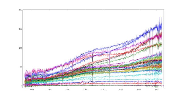
# data from the ith block# function spec_plot() to extract and plot the spectrum of a fits file.
>>> import pyfits as pf
>>> plot.hold(True)
>>> spec_plot(file):
... hdulist = pf.open(file)
... print hdulist.info()
... print len(hdulist[1].data)
... flux = []
... loglam = []
... for i in xrange(len(hdulist[1].data)):
... tmp = (hdulist[1].data)[1][0:1]
... flux.append(tmp)
... temp = (hdulist[1].data)[1][1:2]
... loglam.append(temp)
# in this specific case, the 1st block contains the data pertaining to the spectrum and the 1st value in this block is flux while the 2nd value is the log(lambda)
... print len(flux)
... print len(loglam)
... plot(loglam, flux, lw=0.3)>>> plt.hold(True)$ ls >> fits_listthe function read() should be in
/usr/local/lib/python2.7/dist-packages/astropy/io/ascii/basic.py$ locate astropy/io/ascii/basic.pyrdr = ascii.get_reader(Reader=ascii.Basic)
# rdr.header.splitter.delimiter = ' '
rdr.data.splitter.delimiter = ',\n '
# rdr.header.start_line = 0
rdr.data.start_line = 0
rdr.data.end_line = None
# rdr.header.comment = r'\s*#'
# rdr.data.comment = r'\s*#'>>> fin = open('fits_list')
>>> list = fin.readlines()
>>> fin.close()
>>> list[i]
# should explicitly print the ith file name>>> def spec_all(file):
... fin = open(file)
... list = fin.readlines()
... fin.close()
... for k in xrange(len(list)):
... tmp = list[k]
... spec_plot(tmp)
...
>>>| emission line | wavelength(rest frame) |
|---|---|
| Ly alpha | 1.22E+03 |
| NV 1240 | 1.24E+03 |
| CIV 1549 | 1.55E+03 |
| HeII 1640 | 1.64E+03 |
| CIII] 1908 | 1.91E+03 |
| MgII 2799 | 2.80E+03 |
| OII 3725 | 3.73E+03 |
| OII 3727 | 3.73E+03 |
| NeIII 3868 | 3.87E+03 |
| Hepsilon | 3.89E+03 |
| NeIII 3970 | 3.97E+03 |
| Hdelta | 4.10E+03 |
| Hgamma | 4.34E+03 |
| OIII 4363 | 4.36E+03 |
| HeII 4685 | 4.69E+03 |
| Hbeta | 4.86E+03 |
| OIII 4959 | 4.96E+03 |
| OIII 5007 | 5.01E+03 |
| HeII 5411 | 5.41E+03 |
| OI 5577& | 5.58E+03 |
| OI 6300 | 6.30E+03 |
| SIII 6312 | 6.31E+03 |
| OI 6363 & | 6.37E+03 |
| NII 6548 | 6.55E+03 |
| Halpha | 6.56E+03 |
| NII 6583 | 6.59E+03 |
| SII 6716 | 6.72E+03 |
| SII 6730 | 6.73E+03 |
| ArIII 7135 | 7.14E+03 |